 1
 2
 3
 4
 5
 6
 7
 8
 9
10
11
12
13
14
15
16
17
18
19
20
21
22
23
24
25
26
27
28
29
30
31
32
33
34
35
36
37
38
39
40
41
42
43
44
45
46
47
48
49
50
51
52
53
54
55
56
57
58
59
60
61
62
63
64
65
66
67
68
69
70
71
72
73
74
75
76
77
78
79
80
81
82
83
84
85
86
87
88
89
90
91
92
93
94
95
96
97
98
99
100
101
102
103
104
105
106
107
108
109
110
111
112
113
114
115
116
117
118
119
120
121
122
123
124
125
126
127
128
129
130
131
132
133
134
135
136
137
138
139
140
141
142
143
144
145
146
147
148
149
150
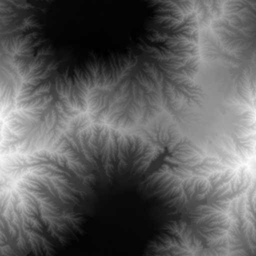
151 | import numpy as np
def lerp(x, y, a): return (1.0 - a) * x + a * y
def simple_gradient(a):
dx = 0.5 * (np.roll(a, 1, axis=0) - np.roll(a, -1, axis=0))
dy = 0.5 * (np.roll(a, 1, axis=1) - np.roll(a, -1, axis=1))
return 1j * dx + dy
def displace(a, delta):
fns = {
-1: lambda x: -x,
0: lambda x: 1 - np.abs(x),
1: lambda x: x,
}
result = np.zeros_like(a)
for dx in range(-1, 2):
wx = np.maximum(fns[dx](delta.real), 0.0)
for dy in range(-1, 2):
wy = np.maximum(fns[dy](delta.imag), 0.0)
result += np.roll(np.roll(wx * wy * a, dy, axis=0), dx, axis=1)
return result
def gaussian_blur(a, sigma=1.0):
freqs = tuple(np.fft.fftfreq(n, d=1.0 / n) for n in a.shape)
freq_radial = np.hypot(*np.meshgrid(*freqs))
sigma2 = sigma**2
g = lambda x: ((2 * np.pi * sigma2) ** -0.5) * np.exp(-0.5 * (x / sigma)**2)
kernel = g(freq_radial)
kernel /= kernel.sum()
return np.fft.ifft2(np.fft.fft2(a) * np.fft.fft2(kernel)).real
def normalize(x, bounds=(0, 1)):
return np.interp(x, (x.min(), x.max()), bounds)
def fbm(shape, p, lower=-np.inf, upper=np.inf):
freqs = tuple(np.fft.fftfreq(n, d=1.0 / n) for n in shape)
freq_radial = np.hypot(*np.meshgrid(*freqs))
envelope = (np.power(freq_radial, p, where=freq_radial!=0) *
(freq_radial > lower) * (freq_radial < upper))
envelope[0][0] = 0.0
phase_noise = np.exp(2j * np.pi * np.random.rand(*shape))
return normalize(np.real(np.fft.ifft2(np.fft.fft2(phase_noise) * envelope)))
def sample(a, offset):
shape = np.array(a.shape)
delta = np.array((offset.real, offset.imag))
coords = np.array(np.meshgrid(*map(range, shape))) - delta
lower_coords = np.floor(coords).astype(int)
upper_coords = lower_coords + 1
coord_offsets = coords - lower_coords
lower_coords %= shape[:, np.newaxis, np.newaxis]
upper_coords %= shape[:, np.newaxis, np.newaxis]
result = lerp(lerp(a[lower_coords[1], lower_coords[0]],
a[lower_coords[1], upper_coords[0]],
coord_offsets[0]),
lerp(a[upper_coords[1], lower_coords[0]],
a[upper_coords[1], upper_coords[0]],
coord_offsets[0]),
coord_offsets[1])
return result
def apply_slippage(terrain, repose_slope, cell_width):
delta = simple_gradient(terrain) / cell_width
smoothed = gaussian_blur(terrain, sigma=1.5)
should_smooth = np.abs(delta) > repose_slope
result = np.select([np.abs(delta) > repose_slope], [smoothed], terrain)
return result
def erode(heightmap: np.array, cycles=1.0):
full_width = heightmap.shape[0]
dim = heightmap.shape[0]
shape = heightmap.shape
cell_width = full_width / dim
cell_area = cell_width ** 2
# Generate terrain from noise
#heightmap = fbm(shape, -2.0)
water = np.zeros_like(heightmap)
velocity = np.zeros_like(heightmap)
sediment = np.zeros_like(heightmap)
# Water constants
rain_rate = 0.0008 * cell_area
evaporation_rate = 0.0005
# Slope constants
min_height_delta = 0.05
repose_slope = 0.03
gravity = 30.0
gradient_sigma = 0.5
# Sediment constants
sediment_capacity_constant = 50.0
dissolving_rate = 0.25
deposition_rate = 0.001
for _ in range(int(1.4*dim*cycles)):
water += np.random.rand(*shape) * rain_rate
# Compute normalized gradient
gradient = np.zeros_like(heightmap, dtype='complex')
gradient = simple_gradient(heightmap)
gradient = np.select(
[np.abs(gradient) < 1e-10],
[np.exp(2j * np.pi * np.random.rand(*shape))],
gradient
)
gradient /= np.abs(gradient)
# Compute the difference between the current height and the
# height offset by the gradient
neighbor_height = sample(heightmap, -gradient)
height_delta = heightmap - neighbor_height
# See the notes about this equation in a previous section.
sediment_capacity = ((np.maximum(height_delta, min_height_delta) / cell_width) * velocity * water * sediment_capacity_constant)
deposited_sediment = np.select(
[
height_delta < 0,
sediment > sediment_capacity,
], [
np.minimum(height_delta, sediment),
deposition_rate * (sediment - sediment_capacity),
],
dissolving_rate * (sediment - sediment_capacity)
)
deposited_sediment = np.maximum(-height_delta, deposited_sediment)
sediment -= deposited_sediment
heightmap += deposited_sediment
sediment = displace(sediment, gradient)
water = displace(water, gradient)
# Smooth out steep slopes
heightmap = apply_slippage(heightmap, repose_slope, cell_width)
# Update velocity
velocity = gravity * height_delta / cell_width
# Apply evaporation
water *= 1 - evaporation_rate
return heightmap
#pyplot.imsave("/static/erosion_imgs/efficient1.png", erode(fbm([512, 512], -2)), cmap='grey')
|